|
A primer on the
three dimensional complex numbers.
|
| Introduction: This
file is a collection of the pictures from Feb 2012 until now that are
related to the 3D complex numbers. 3D complex numbers are in many ways just like the ordinary complex numbers from the complex plane; only in the 3D case you simply 'create' an 'imaginary number' j who's third power equals minus one. Recall that in the ordinary complex plane the 'imaginary unit' i has a square of minus one. Just like ordinary complex numbers (written often as z = x + iy) it looks rather elementary to use rectangular coordinates in real numbers (x, y, z). Therefore the number one is
written as 1 = (1, 0, 0) __________ So only pictures in this stuff below... Remark: Everywhere where in these pictures it says 'see below' you must read that as 'see above' in some other picture. (Because this file is chronological while the homepage of this website is anti-chronological.) |
|
|
|
|
| From 13
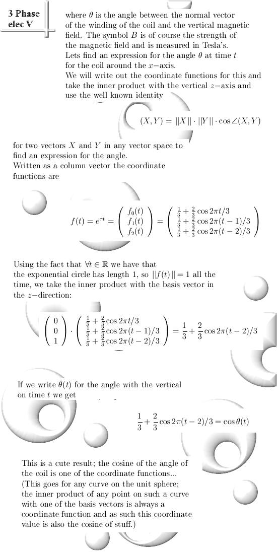
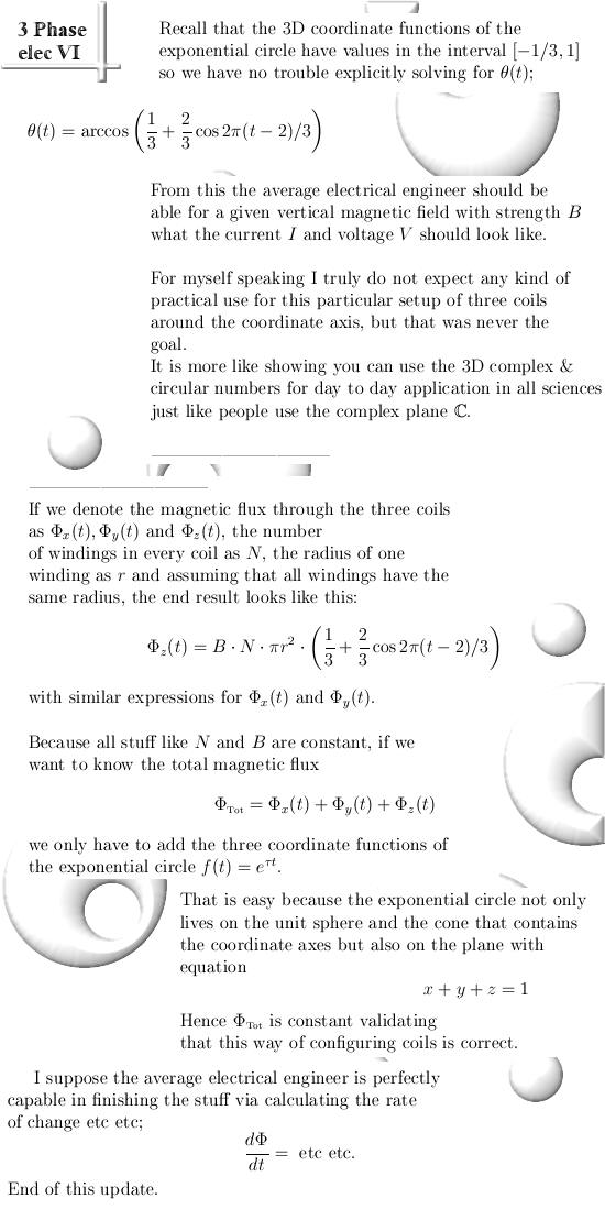
Feb 2015: 3 phase electricity and 3D circular numbers.
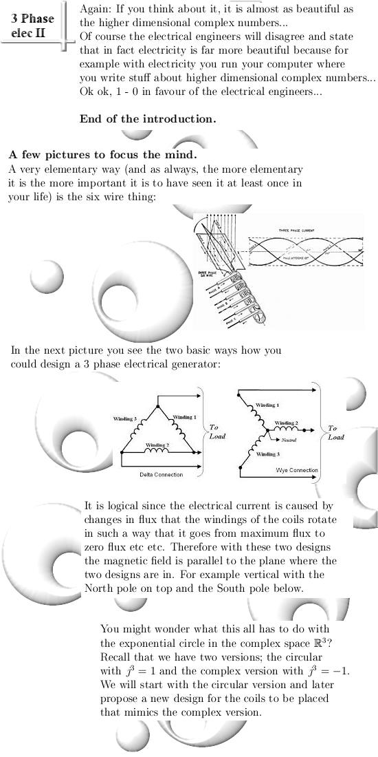
This update contains no new mathematics but the goal is to show that you can apply the higher dimensional complex and circular numbers to almost everything just like it is always done with complex numbers from the complex plane. Industrial electricity or 3 phase electricity is just screaming bloody murder for 3D numbers, just look at the way the voltages behave and you understand why. In this update I propose a new design for the placement of the coils, as far as I can see this will have no serious practical application anywhere, but once more: I want to show you that there is no reason to skip 3D numbers in practical applications... Enough of the bla bla introduction, here is the six page long update:
Once more: this update only serves as an example that you can use 3D numbers just as easily as 2D complex numbers or 1D real numbers... Till updates.
|
| From 23
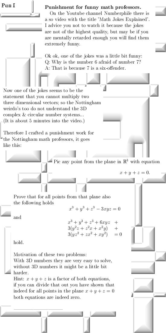
Feb 2015: Punishment for funny Nottingham professors.
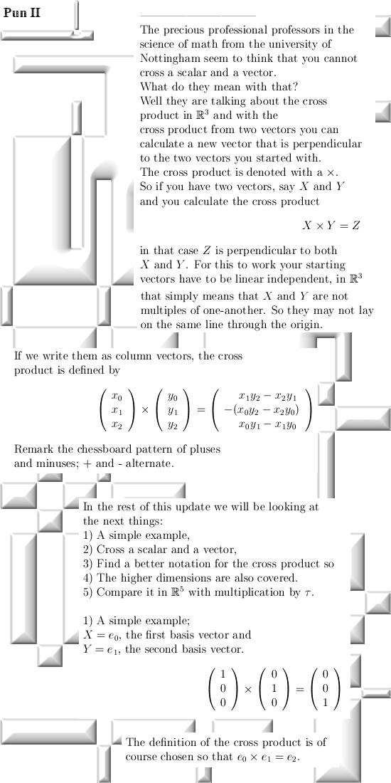
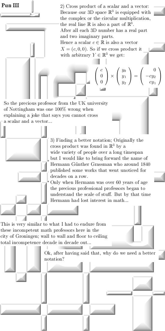
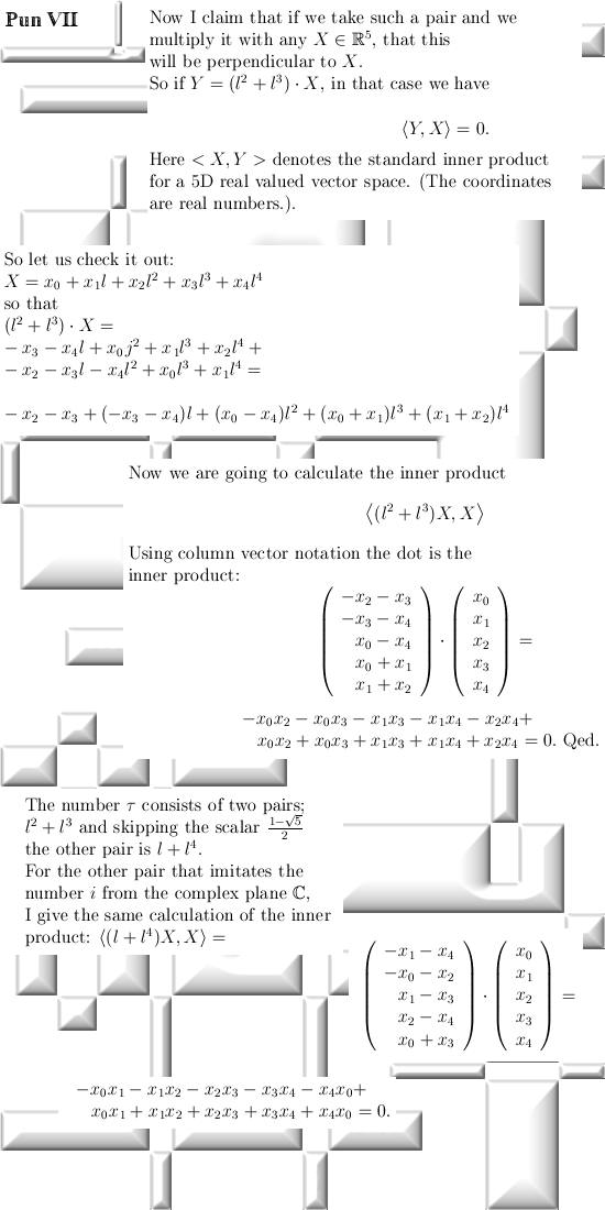
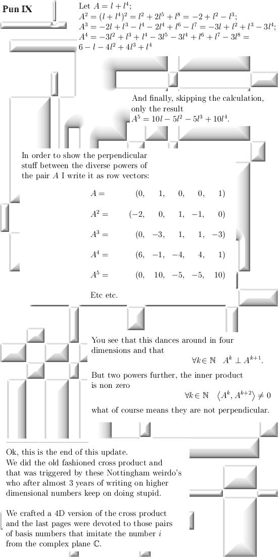
Almost 3 years of writing on higher dimensional complex & circular numbers & of course the Nottingham professors still do not have any clue whatsoever... Anyway, at the Nottingham university they have those Numberphile video series and one of them is about math humor. In that it was stated that you cannot take the cross product of a scalar and a vector and that was viewed upon as a joke. Later I realized once more how dumb and retarded you become when rejecting that large ocean of math known as the higher dimensional numbers. But Nottingham is not the only university, the sleazeballs from my own university here in Groningen do a perfct job hanging out the silent coward. Well, apparently that is the choice they have made... __________ In this update: The good old cross product in
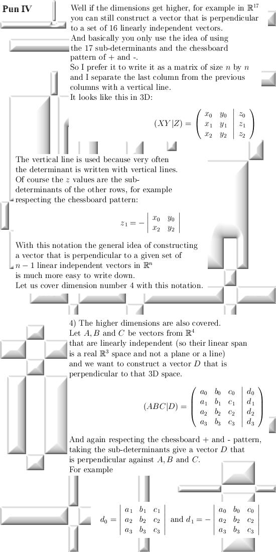
3D plus a 4D version of it. Let's get started:
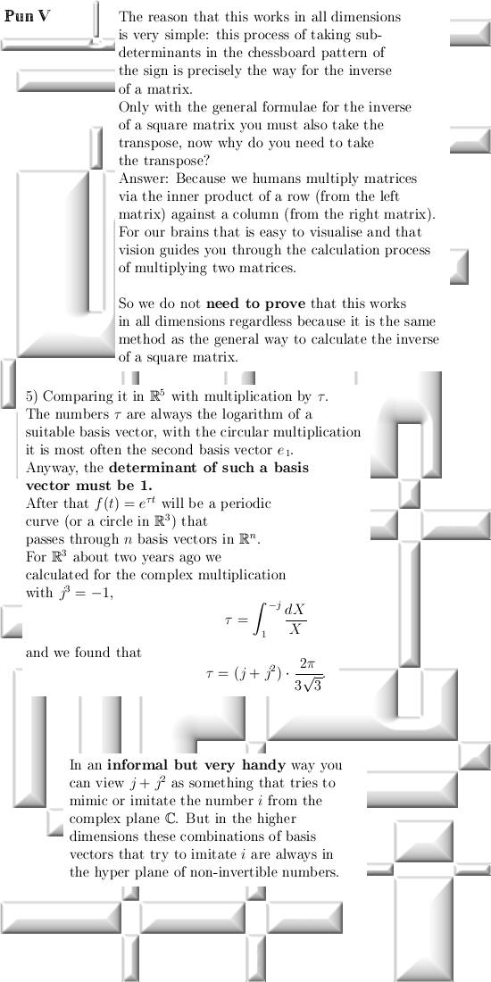
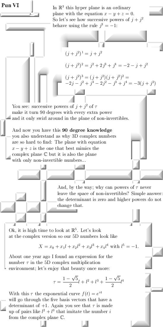
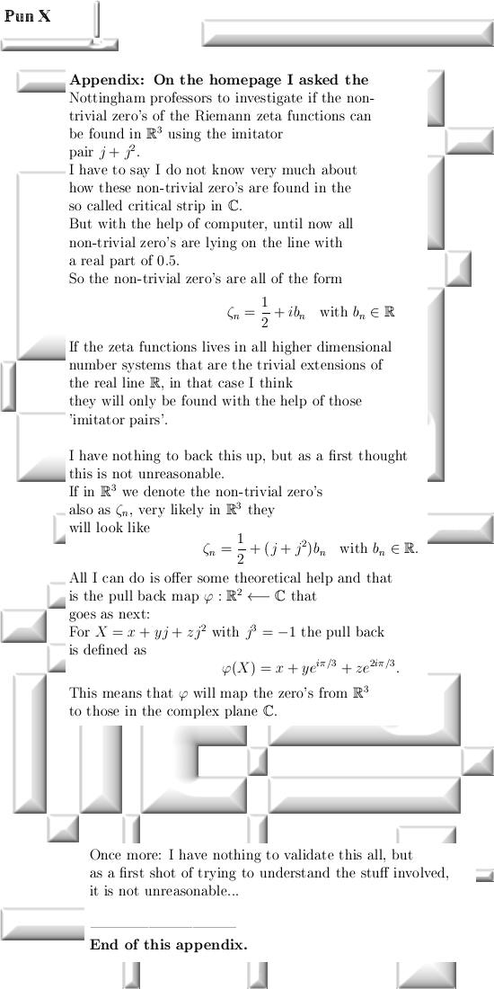
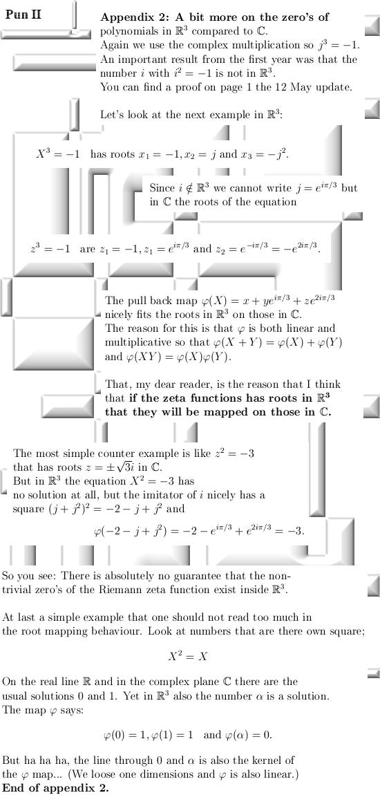
In the second appendix we look a bit deeper into why this root mapping stuff between different dimensions actually works. Here is appendix number two:
End of this update, till updates.
|
| From 05
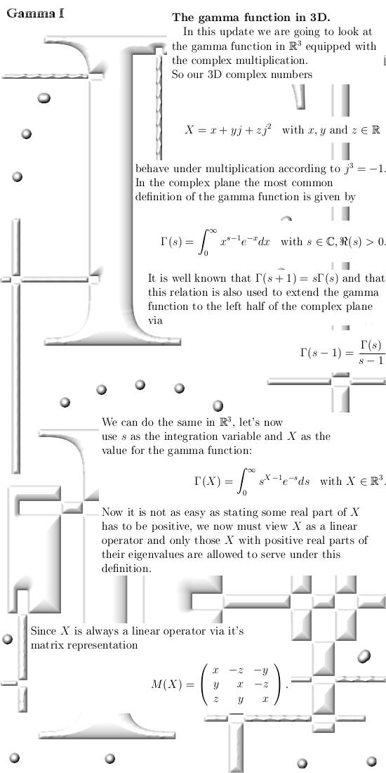
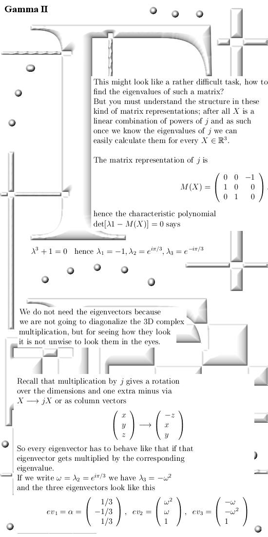
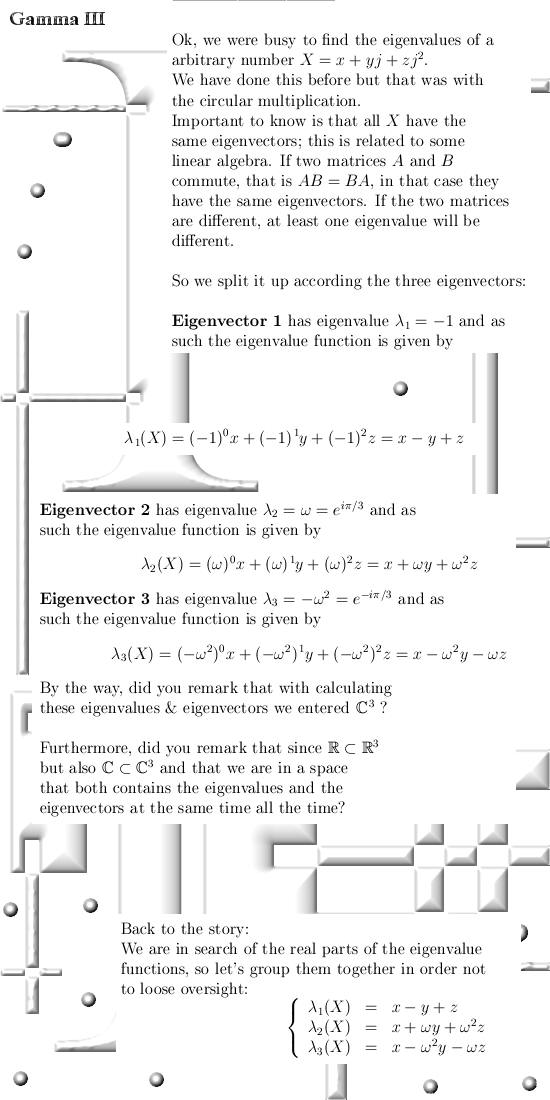
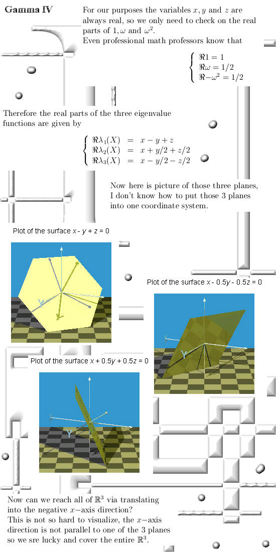
March 2015: The gamma function in 3D (using the complex
multiplication in 3D, the circular multiplication goes similar).
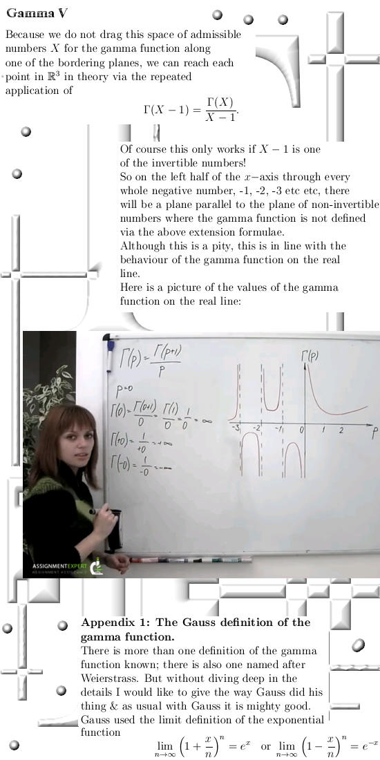
All functions that are analytic on the real line can be extended to three dimensional complex space; in the previous update I did that for the Riemann zeta function, in this update we take a look at the gamma function. Here we go, it is seven pages long:
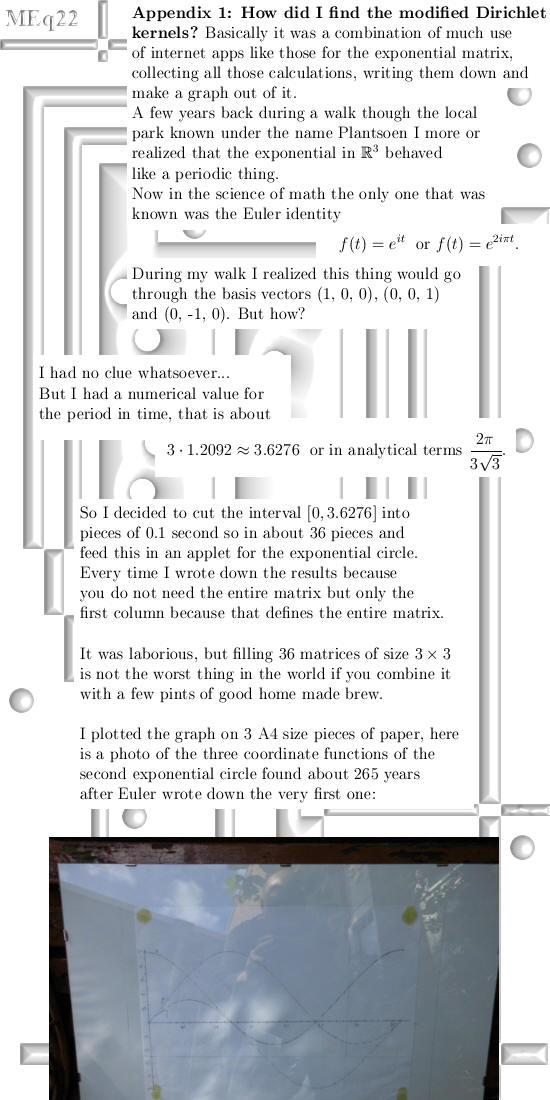
I did not change one little
detail at that Gauss representation thing, normally I never include stuff
from other math folks unchanged but for Gauss I make an exception because
Gauss was just like me a math amateur. Here is the link to the Youtubber: Gamma
Function - Part 2 - Gauss Representation Also including much info on the gamma function in one & two dimensions: Gamma
function __________ End of this update. Till updates.
|
|
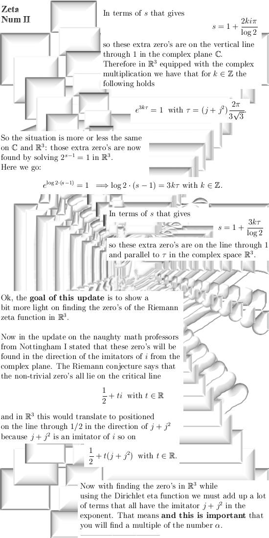
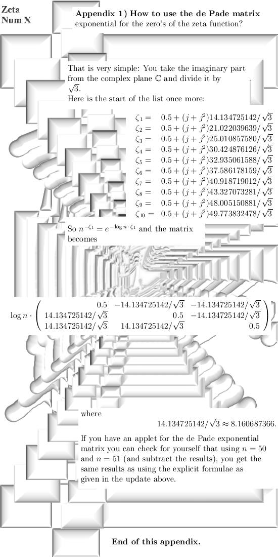
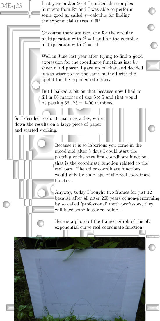
From 26 March 2015: Zeta on the critical strip (3D version only). This update is about numerical
math to find the zero's of the Riemann zeta function in 3D. For myself speaking, I think
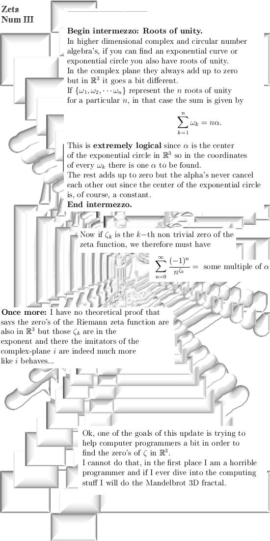
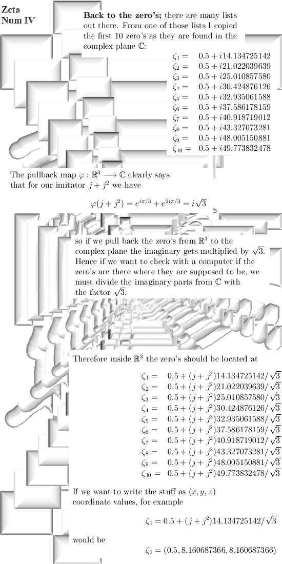
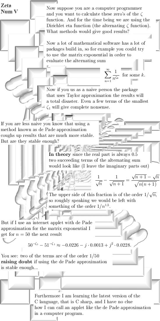
the zero's are also on a critical line in 3D complex space. Because all universities completely neglect me, I have no access to reliable computers. Therefore I have no clue if my insights are indeed correct, but if they are correct you should find multiples of the number alpha on the places a Riemann zeta zero is expected. Despite the coward and
retarded behavior of the 'official universities', for me it was fun to
write a bit into the direction of numerical math. But I refuse to write
computer code to find the zero's of the Riemann zeta function; how can a
reasonable person trust the Microsoft C sharp language? __________ Enough of the introductionary bla bla, this update is nine pages long. Here we go:
A small appendix telling you the obvious: End of this update.
|
| From 06
April 2015: When thinking about the Stern Gerlach experiment
where ionized silver atoms were send through an inhomogeneous magnetic
field, I suddenly thought; this can only happen if the electrons are
magnetic monopoles.
Because if they were magnetic dipoles, because of their very little weight they would always align themselves towards the stronger part of the inhomogeneous magnetic field. So the outcome of the amazing Stern Gerlach experiment can perfectly be explained if electrons were in fact magnetic monopoles. Once you are on that track, you realize soon that if electrons were magnetic dipoles if would be very strange to observe only pairs of electrons; with ordinary bar magnets you can make circles of magnets with any kind of number. For example 3 bar magnets in an equilateral triangle. If you would have a triple electrons, on one side you can put a hydrogen nucleus (a proton) and at the other side a helium nucleus to form HHe or the well known helium hydrogen molecule... Of course this molecule does not exist because as a matter of fact Helium is one of the inert gasses because the outer orbital is completely filled with electron pairs. Nowhere in the last year or this year I have found one little piece of evidence that electrons are magnetic dipoles; ok ok if the are in orbit they create the standard dipole magnetic field that comes with electrical currents that circle around. But on there own electrons are magnetic monopoles. Anyway, that is what I think of it. __________ Now what pushed me over the edge in penning these two pages down is an article I found via the website of CERN; it is available at the preprint archive and has the title: The Search for Magnetic
Monopoles. In the article I found on what equation Dirac concluded that if a magnetic monopole does exist, in that case all electrical forces would be quantasized. That is: all electrical charges come in multiples on one smallest charge. The charge of an electron is often denoted as e, we know now that quarks have charges of e/3 and 2e/2. So for the time being this smallest charge possible is e/3 and all other charges in our macroscopic would are multiples of that... __________ After this long introduction, here are the two pages of this update:
An important detail: if
electrons are in fact magnetic monopoles, one of the laws of Gauss about
magnetism is no longer valid. I do not want to discredit Gauss in any way; he was a great guy because just like me he did not want any kind of career in professional mathematics because basically these are all retards. Although highly intelligent, all these math professors only serve their masters and are afraid to think outside the box. The average math professor is only worried about what the colleagues would think and because of that fundamental emotional hinder they perform far beyond their potential. __________ May be my vision on professional math is a bit over the top, but with my own skin I have felt how they behave... __________ Links: The
Search for Magnetic Monopoles Also funny is the 'Understanding permanent magnets' from this collection of links: Tech
Notes Till updates.
|
|
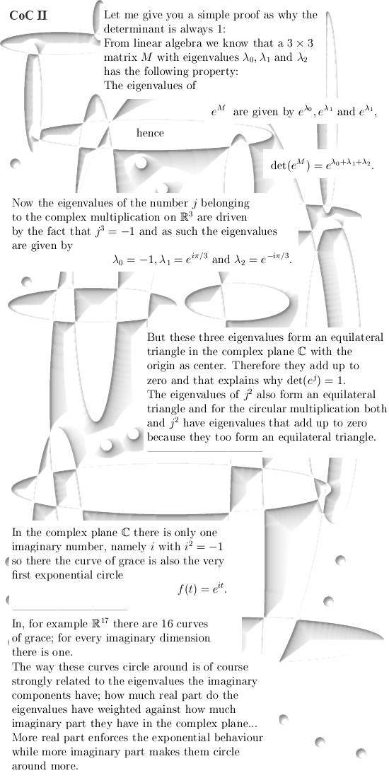
From 18
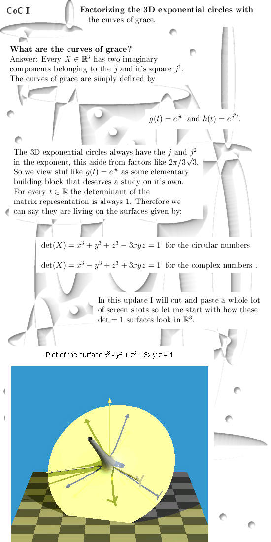
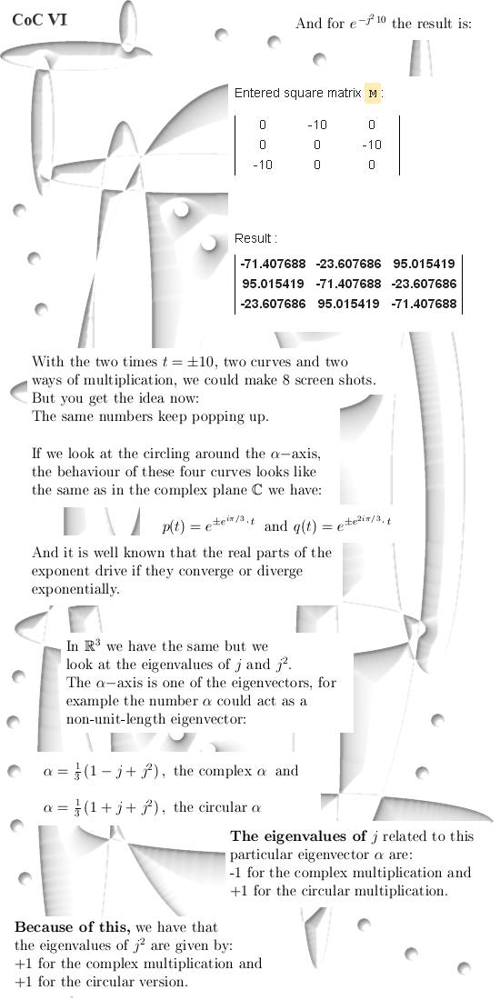
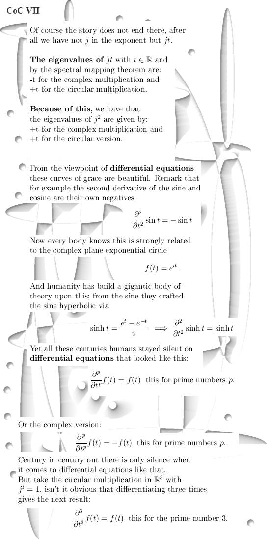
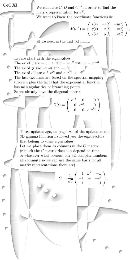
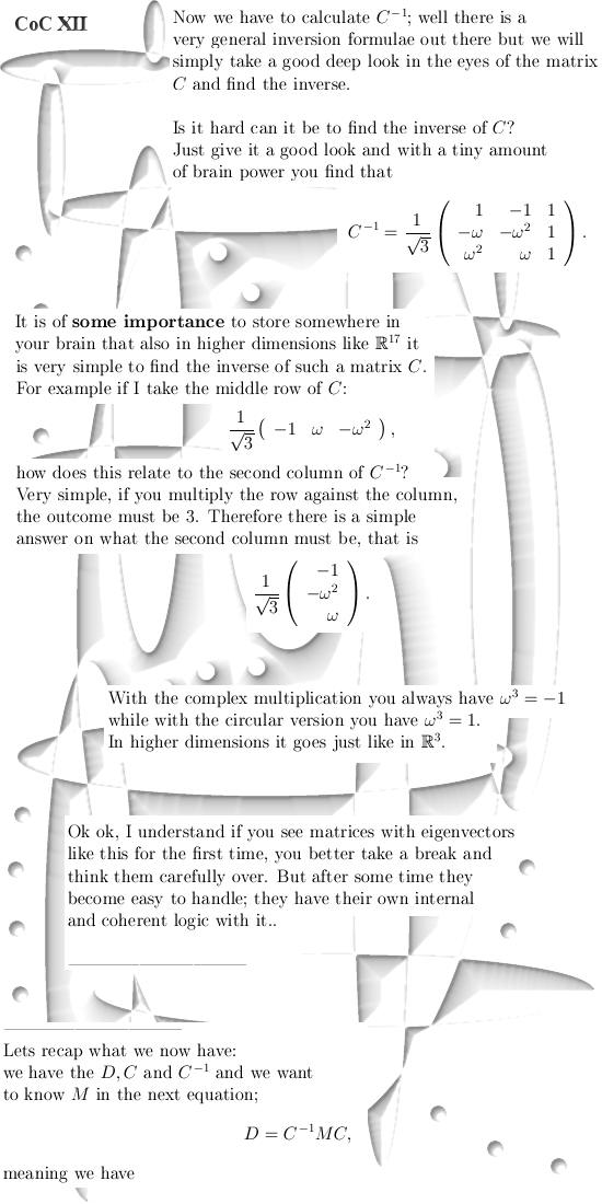
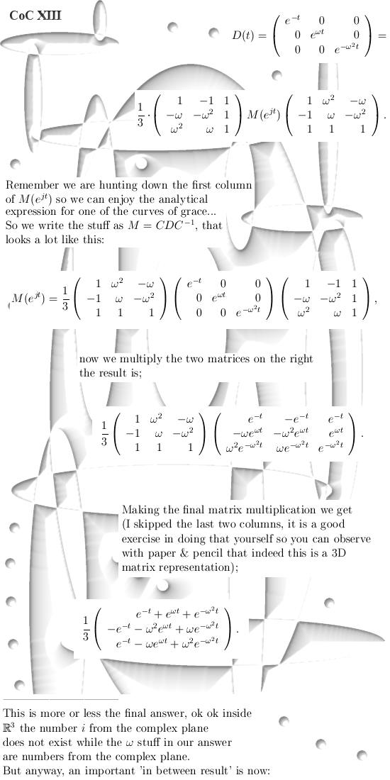
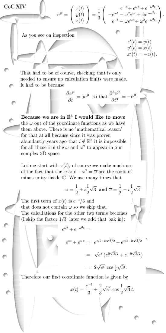
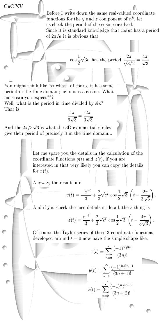
April 2015: The curves of grace in 3D.
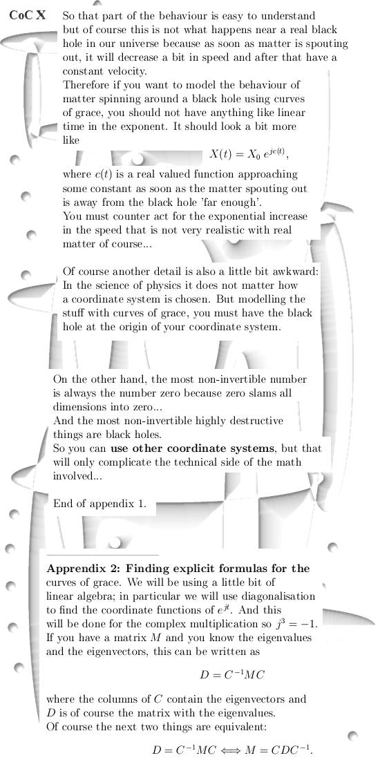
Of course all readers will wonder what ´curves of grace´ are; this is simple to understand:
They are an arbitrary imaginary
number in the exponent and we let run an exponential time evolution.
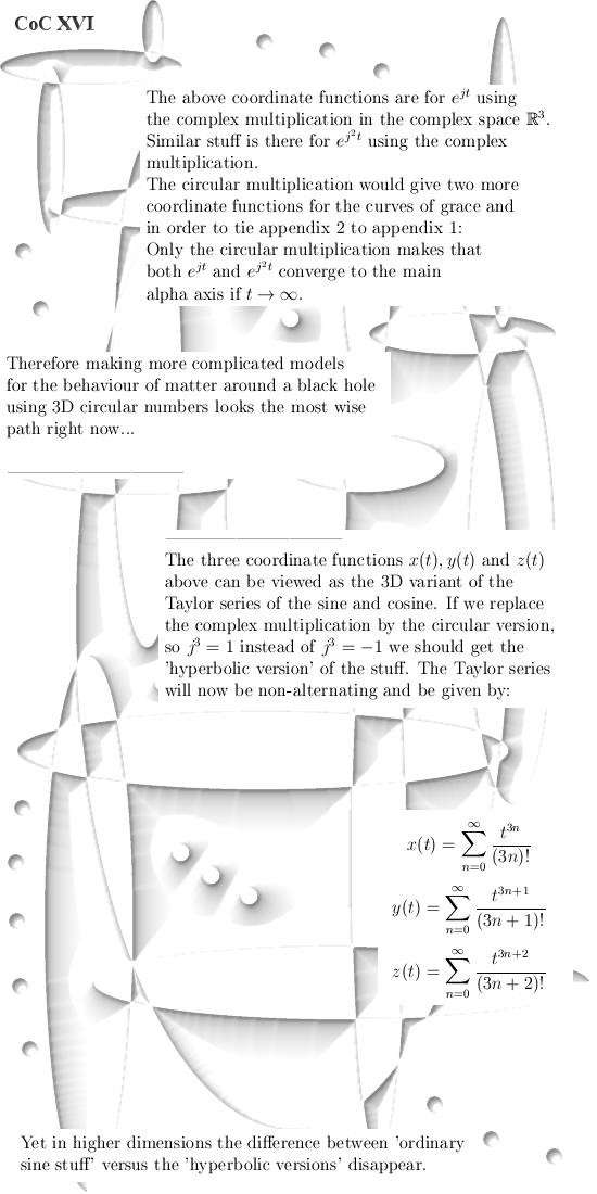
Beside a scaling factor in the
exponent, these curves of grace factorize the exponential circles in 3D.
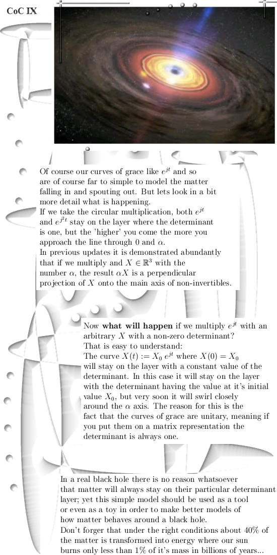
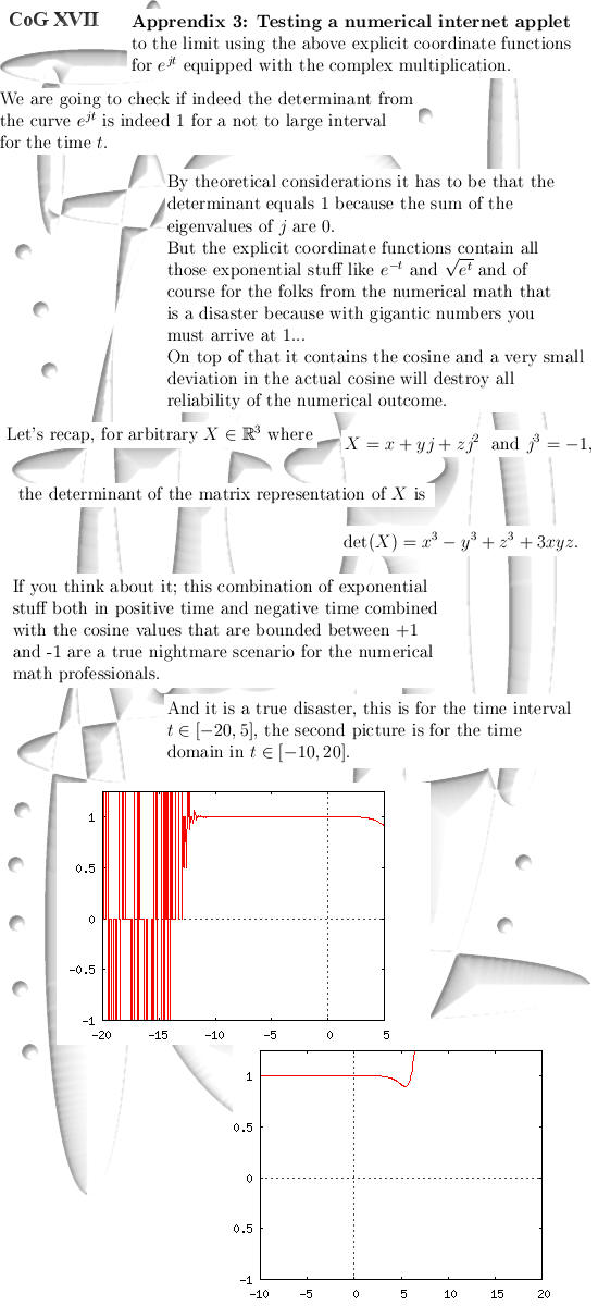
In appendix 1 I propose a very
simple and completely unreliable model for the stream of matter around a
black hole. But that simple flow of matter makes clear to anyone how black
holes probably work. Enough intro talk, here we go:
A few extra words on appendix 1 with the black hole evolutions; Once more realize this simple model is likely far from the truth, yet suppose matter is streaming in along a curve that meets the event horizon of the black hole. That matter will be sucked in. Yet it is important to realize that a black hole and it's event horizon are relatively small objects compared to all that space the in falling matter occupies, so a lot of matter 'will miss' the event horizon. The matter piles up fast and the pressure get tremendously high.
The pressure gets so high that a
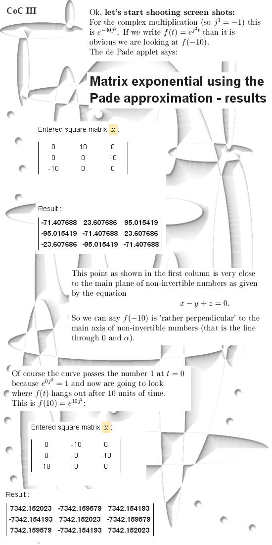
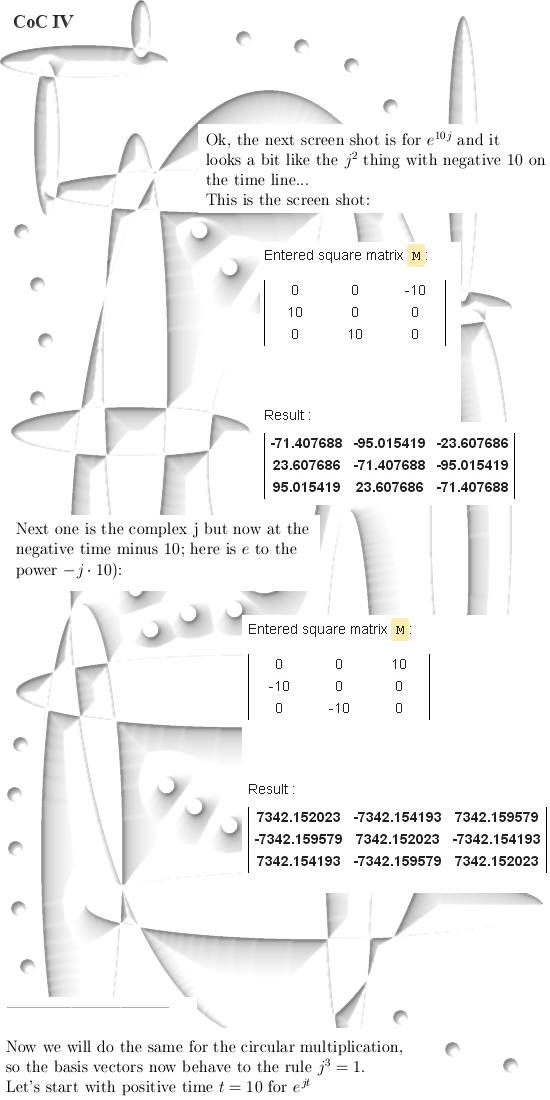
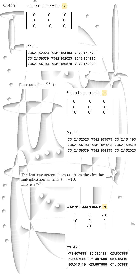
rudimentary version of the Pauli exclusion principle sets in: It is claimed that about 40% of the in falling matter is transformed into energy, I know no way of validating that but if true it is expected it will go more or less as I describe it here: The relatively small size of the event horizon is the main culprit in the building up of the pressure that causes the disintegration of the stuff with mass in it. __________ Used applets: The polyray applet for the
determinant layer on page 1 can be found on: The screen shots for the exponential matrix using the Pade approximation can be found at: Matrix exponential using the Pade approximation calculator __________ The was it for this update, till updates.
|
|
From 08
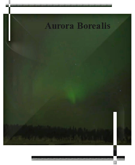
May 2015; The Aurora Borealis and magnetic
monopoles
The Aurora Borealis is the polar light on the Northern hemisphere. In this update that is not on higher dimensional complex numbers but wholly on electrons and protons as being magnetic monopoles. (As a matter of fact I think that all spin half particles are magnetic monopoles.)
The longer I think about it, the
more obvious is that at least electrons are magnetic monopoles. Furthermore, the entire Stern Gerlach experiment was done with ionized electrons; once more if that lonely electron that is unpaired is a magnetic dipole, how can only one electron steer the entire silver ion away from the stronger parts of the magnetic field. __________
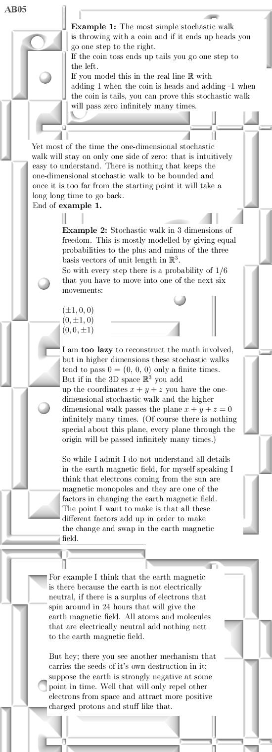
In this update we will do two so
called thought experiments; we pretend to be an electron coming from the sun
via the solar wind and we will be either a bipolar magnetic thing and a
monopole magnetic thing. It is five pages long, at the end I give two simple stochastic walks because I view the earth magnetic field as some giant complicated stochastic walk. We try to shine a bit of light on why the earth magnetic field is always changing direction over the millennia. But it is a geological fact the earth magnetic field always changes in a rather chaotic fashion... Here are the five pages:
In this update I avoided all
calculations, yet on the internet there are dozens and dozens files around
that show it could very well be that electrons are magnetic monopoles. Electron
spin resonance (Source BU Chem on Youtube). Electron
spin resonance example (Source BU Chem on Youtube). Hyperfine
coupling (Source BU Chem on Youtube). Zeeman
splitting example 1 (Source BU Chem on Youtube). It is needless to say that in my view the hyperfine spectrum structure is caused by electrons being magnetic monopoles and atomic nuclei are a sum of north and south magnetic monopoles. This also explains why isotopes have different levels of spin in there nucleus: the neutron is also the sum of three magnetic monopoles and as such a magnetic monopole... __________ More on the dynamics driving the changes in the earth magnetic field: Geomagnetic
reversal (Source WikipediA) 2012: Magnetic Pole Reversal Happens All The (Geologic) Time
(Source NASA) __________ Let me end this update with a picture for this update, it is from a video from the Aurora Borealis: Ok, that was it for this update. Till updates.
|
|
From 14
June 2015: Strong Interaction and 3D circular numbers.
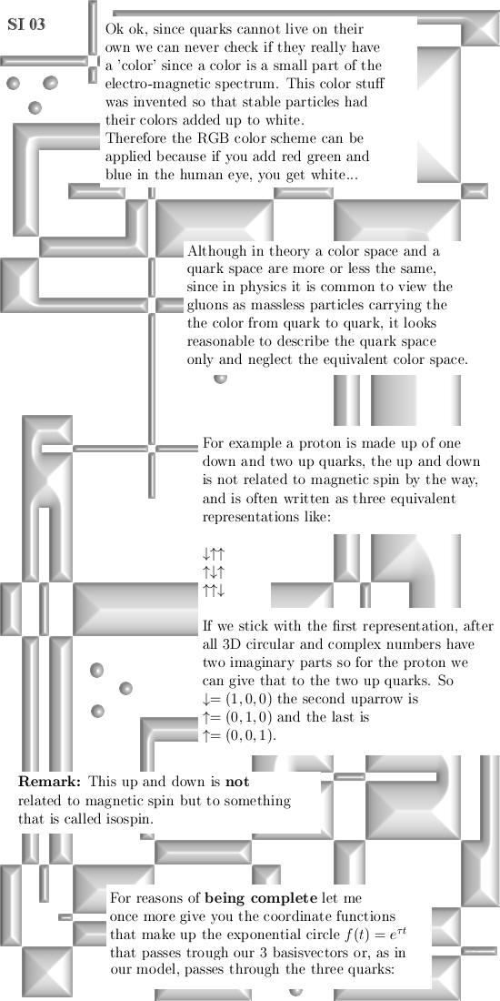
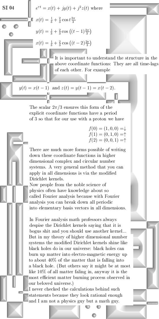
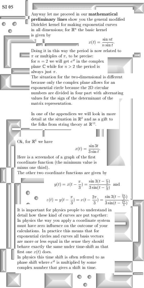
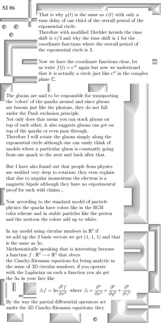
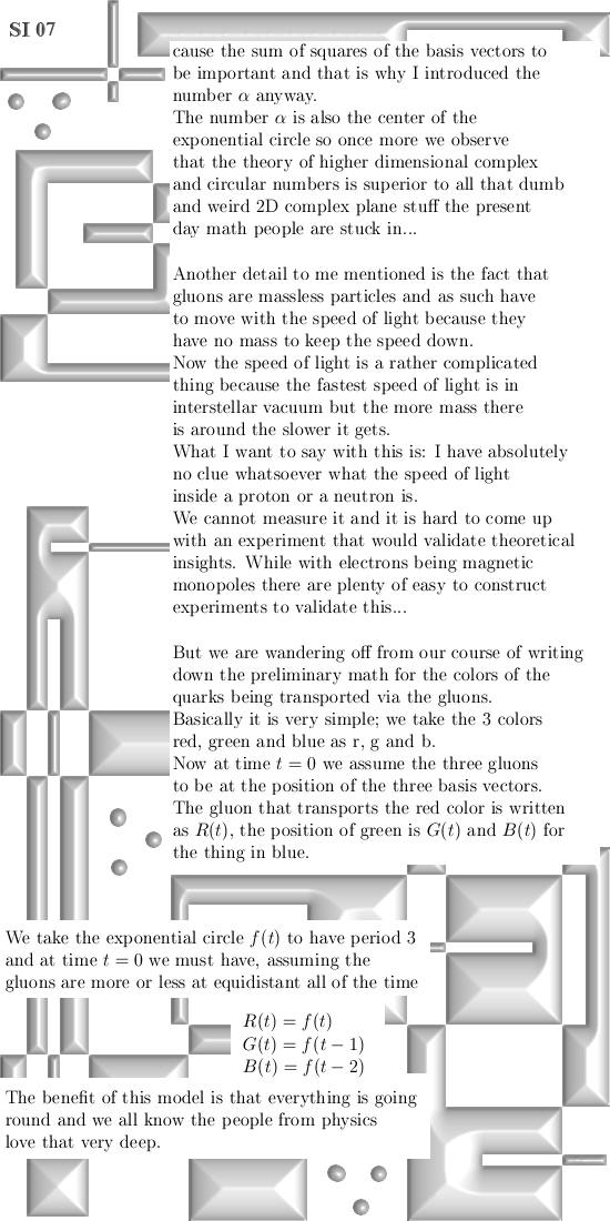
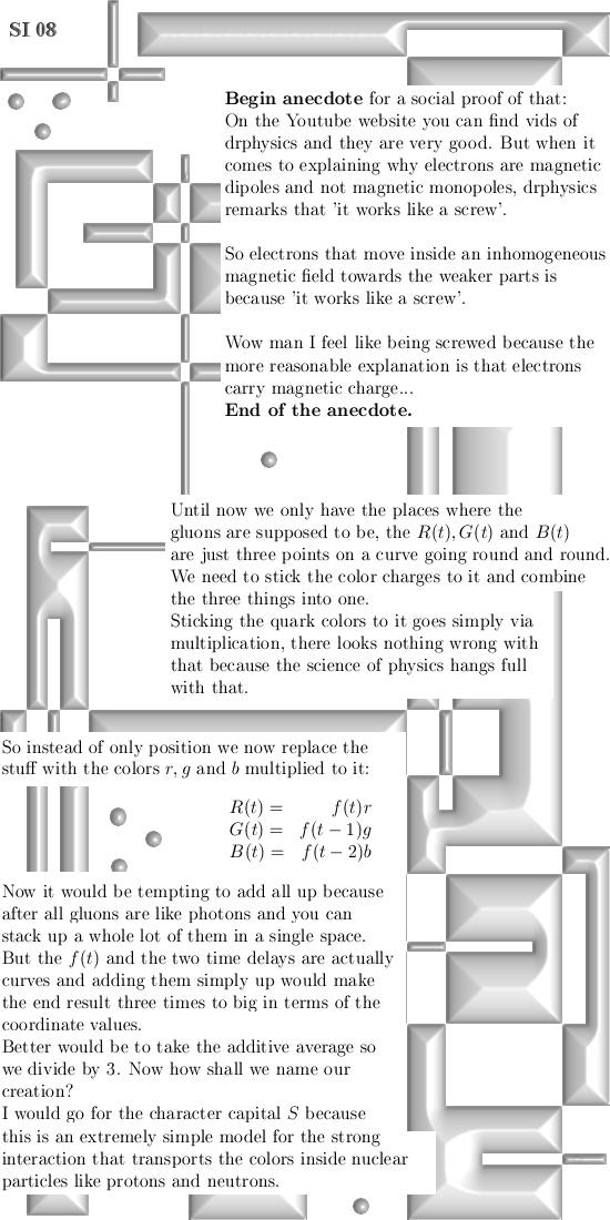
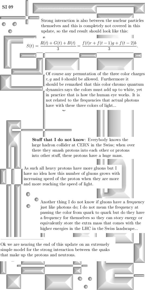
The strong interaction is what the protons and neutrons bind into nuclear particles and via the exchange of pions it holds the nucleus together. That is why relatively small nuclei are so strong compared to large and-or instable nuclei because those are hold together by the electro/magnetic forces. How this last thing actually happens is never good explained by the people of physics because according to the standard model of particle physics spin half particles are not magnetic monopoles... This update is only about the strong interaction inside the proton and the neutron and it is 15 pages long and has three appendices at the end. By sheer coincidence I did
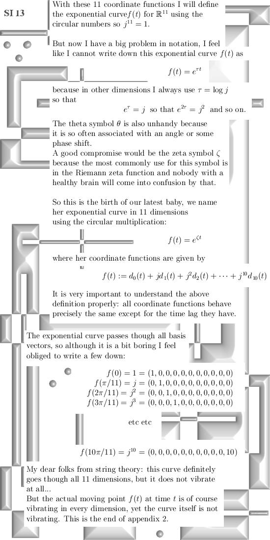
include the exponential curve for the 11-dimensional real space equipped
with the circular multiplication. That was meant as comparisment to the
folks from string theory that use vibrating strings to explain everything;
tiny problem is that the scale where these vibrating strings operate are
completely outside experimental validation. The simple model as I craft it
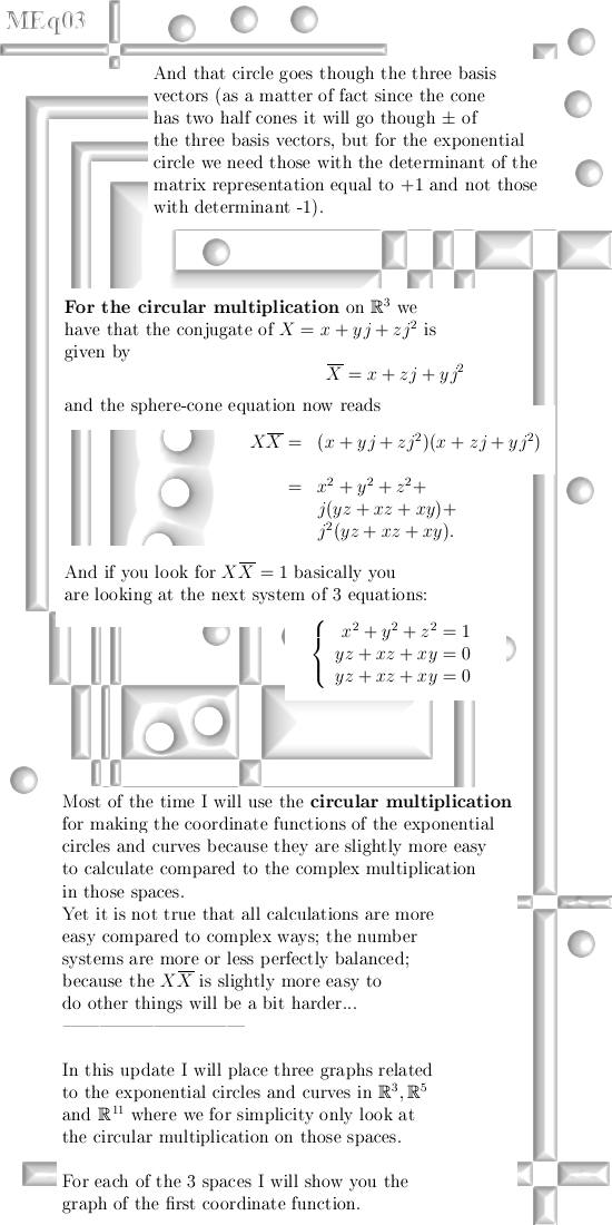
here is the 3D exponential circle that passes through the three basis
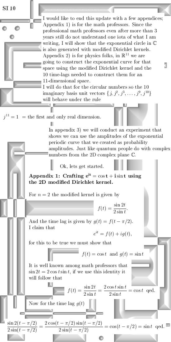
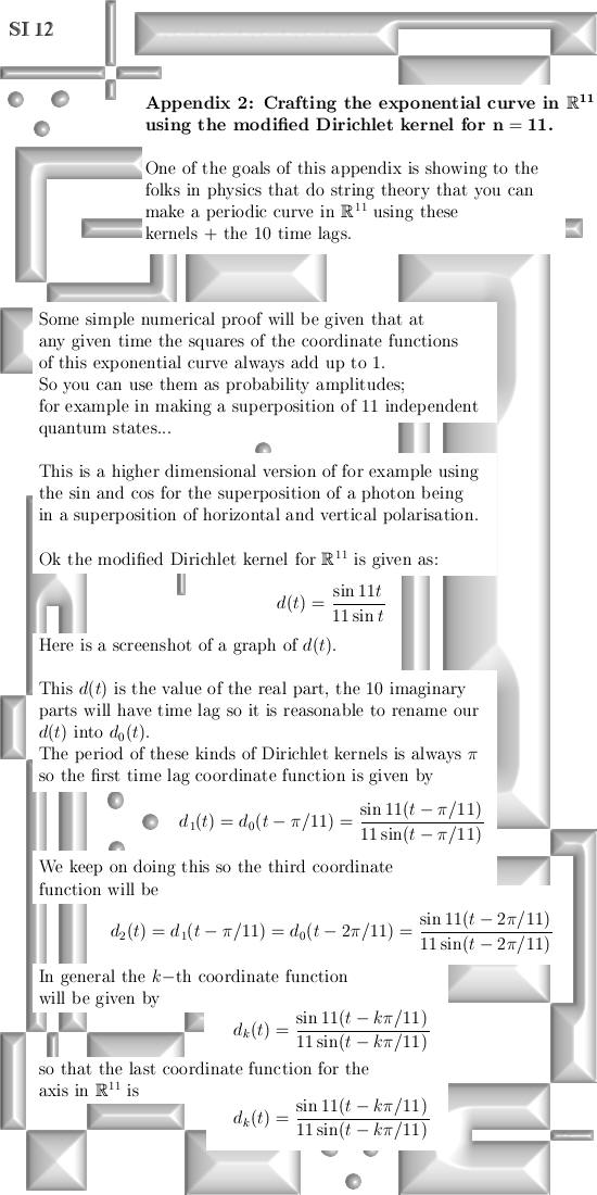
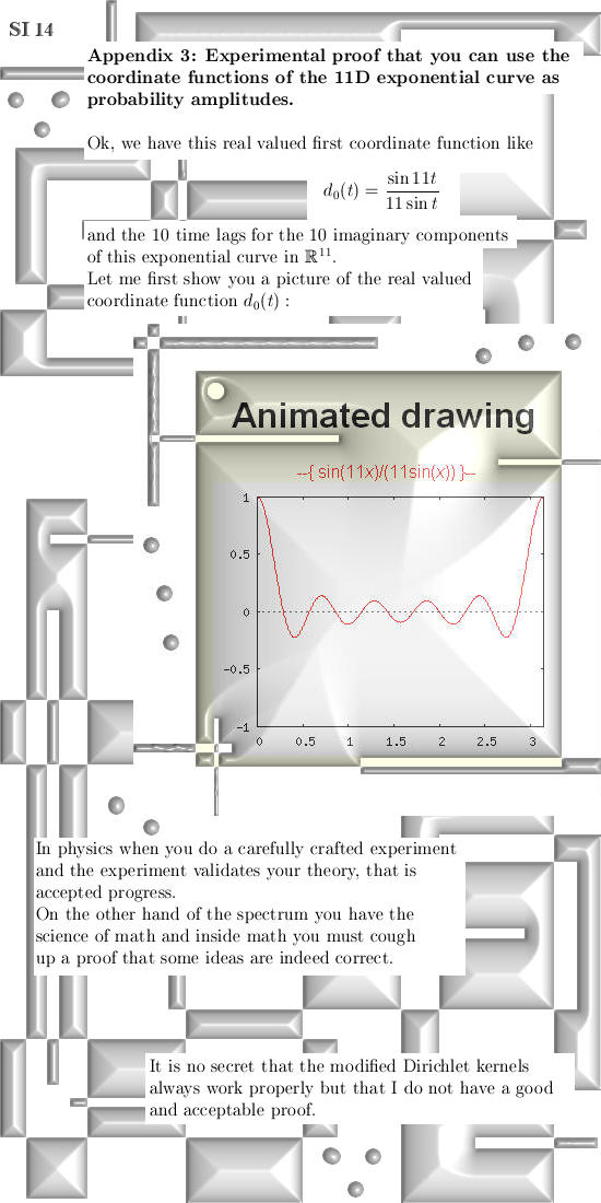
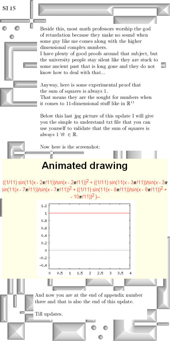
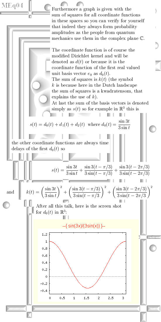
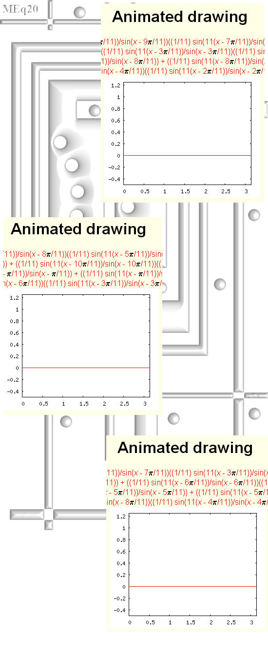
vectors So you can view this update as one the things you can do with exponential circles and curves. In the appendices I give also a way to construct the exponential circle from the complex plane using 2D modified Dirichlet kernels and in the last appendix there is experimental proof you can use the 11D exponential curve as probability amplitudes as they do in quantum physics. All in all this update is much more mathematical physics and not pure math; but that is ok because every now and then some applications must come along of course. Let's get started; 15 pictures on A4 size:
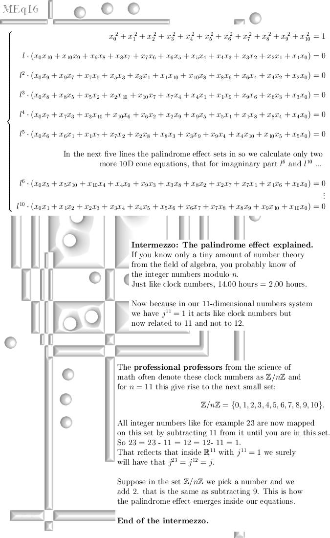
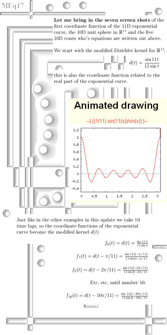
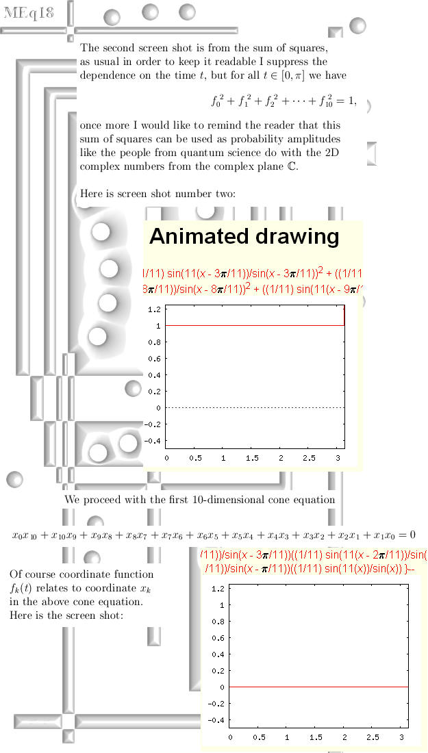
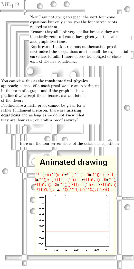
You can use the next text with a bit of cut and paste in order to check that the above math experiment is indeed correct and you can use the values of the coordinate functions as probability amplitudes because the squares always add up to 1. ((1/11)*sin(11*(x))/sin(x))^2 + You can cut and paste that in some internet application for drawing graphs, I have a strong preference for that WWW Interactive Multipurpose Server or WIMS. They are always session bounded so you must find the applet for yourself but that is not so hard. Here is the link: http://wims.math.leidenuniv.nl/wims/wims.cgi? This is the end of this update, till updates.
|
|
From 14
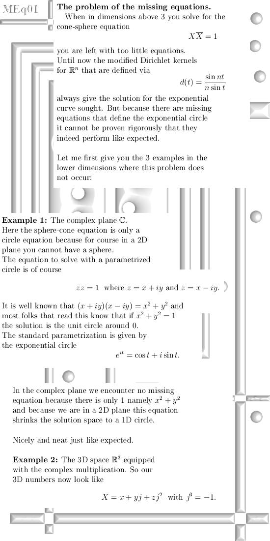
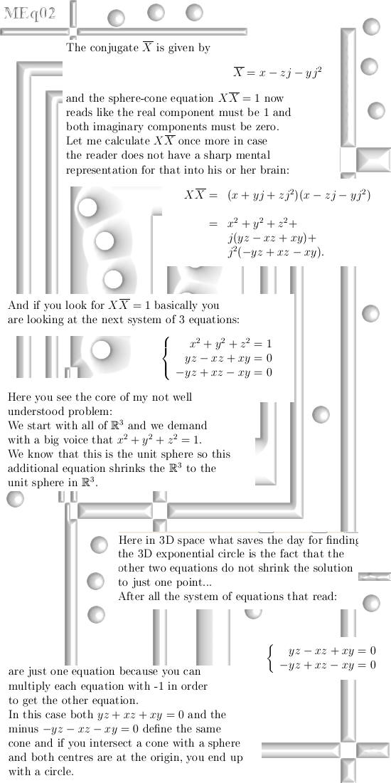
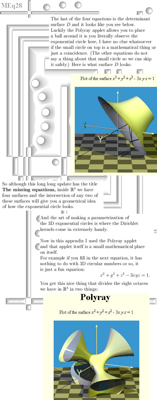
July 2015: The missing equations.
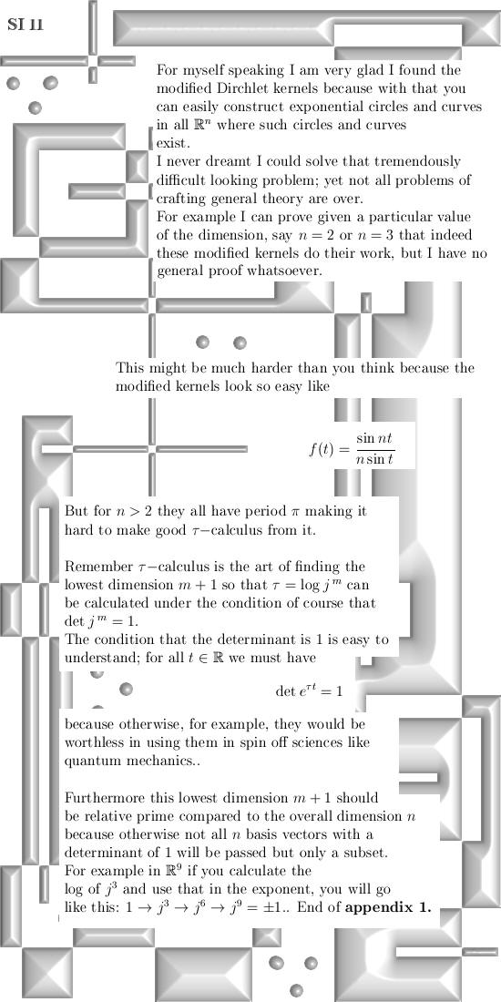
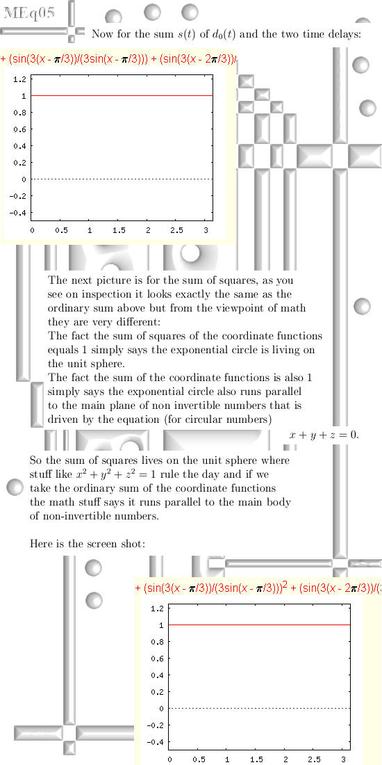
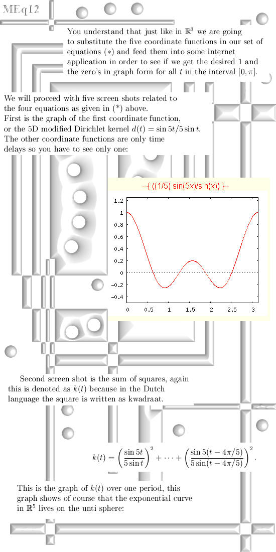
This is a long update of 21 pages; that is an expansion of precisely 10% of all combined updates from the last 3 years although it does not contain 10% more math. This update is more like a physics approach to math; because we have missing equations we simply cannot give mathematical proofs because we do not know what is missing. The equations that we study are those who's solution is an exponential curve, or an exponential circle, and we constantly use the modified Dirichlet kernels to construct the exponential curves/circles. And with each construction we show that from the equations that we know of, they fulfill those equations.
Simple example in the complex
plane: Furthermore we only use internet apps to draw graphs of the parameterizations of our known equations, so in that sense the internet app is the experiment in the science of physics.
Every graph of such an equation in
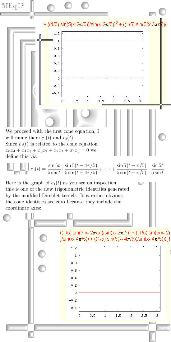
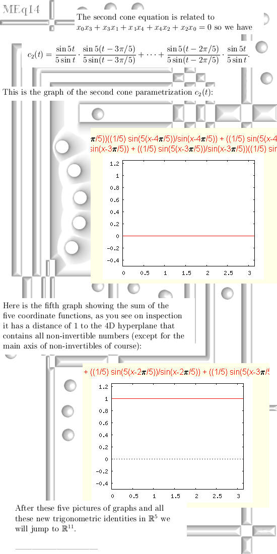
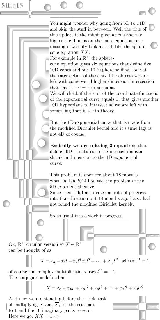
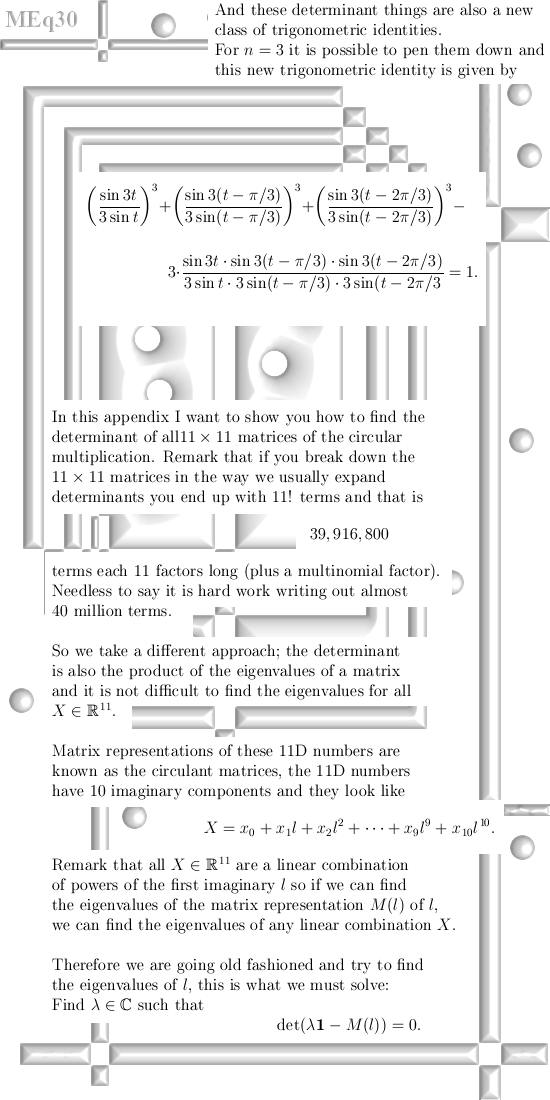
this 21 page update shows a new trigonometric indentity.
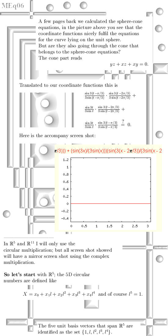
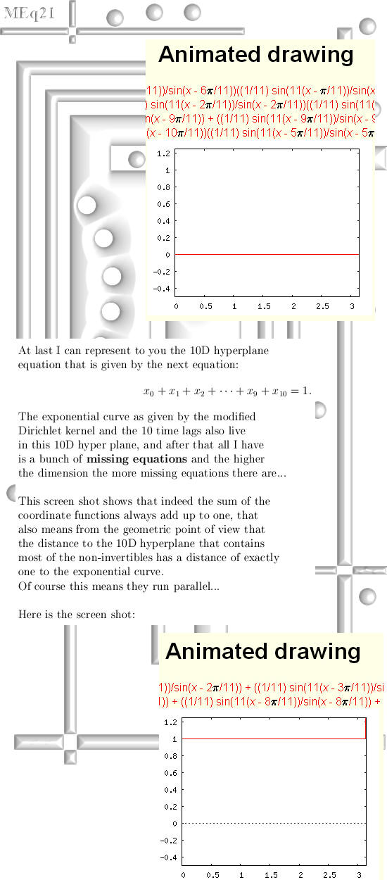
In case you want to make some of those screen shots yourself, you must cut and paste the next stuff that is from the fifth cone equation into the 'Animated drawing' applet in the next link. (Search for graph plotters, 2D explicit variant) and cut & paste this:
((1/11)*sin(11*(x))/sin(x))*((1/11)*sin(11*(x - 6*pi/11))/sin(x - 6*pi/11)) + And the sum of the 11 coordinate functions has the next txt coding:
((1/11)*sin(11*(x))/sin(x)) + The applet ignores the line breaks (the 'return' or 'enter' button from your computer keyboard). The Animated drawing applet can be found here: http://wims.unice.fr/~wims/wims.cgi? __________ May be I will write one or two appendices, if not till updates. __________ Ok ok, on 18 July this is the first appendix where I more or less in detail try to explain how I found the modified Dirichlet kernels. And you can believe me: this modified stuff is awesome...
I guess till the next appendix... __________
And indeed on 20 July 2015 we have
four more pages on the abundance of equations in three dimensional space.
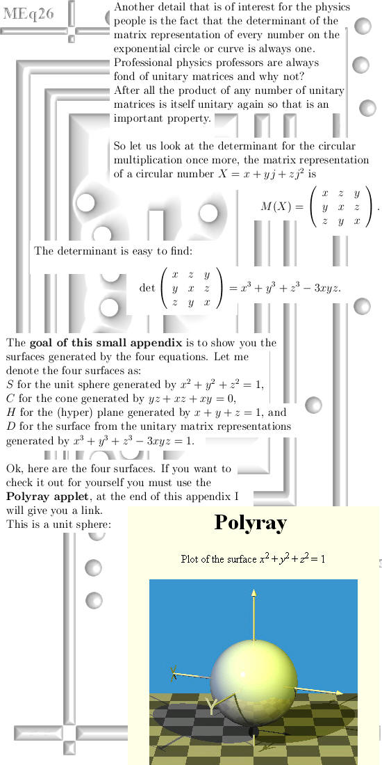
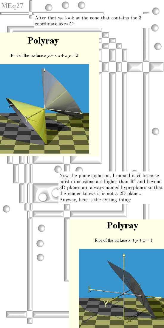
May be I should not have posted the 'fun equation' because it focuses not on higher dimensional complex numbers. Yet it was fun to write it down. Till the next appendix update that will contain only hard core mathematics because after all those fancy screen shots of funny equations it is about time to once more beat the shit out of the math departments on a global scale. So the next and latest appendix will beat some shit out & lets leave it with that. __________ The promised link with the Polyray applet can be found at: The Polyray applet can be found here: http://wims.unice.fr/~wims/wims.cgi? Till updates. __________ On 05 August 2015 there is appendix number 3: Going hardcore nine pages long.
This appendix contains mostly math
so almost no screen shots, to be precise: two screen shots.
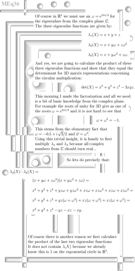
Yet it contains one of the
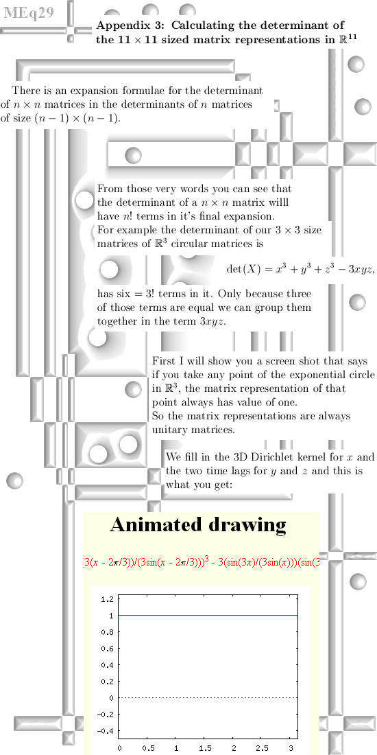
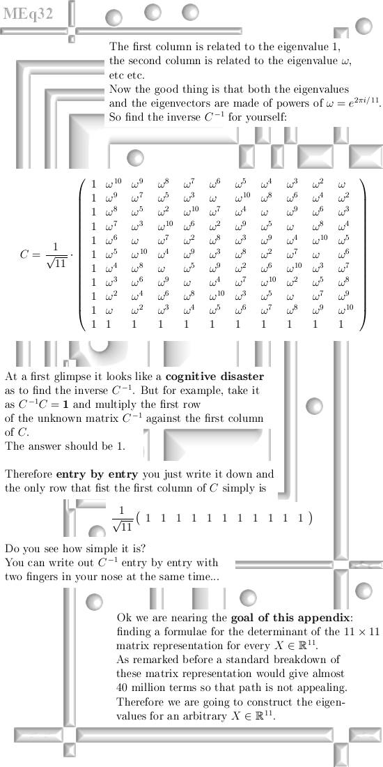
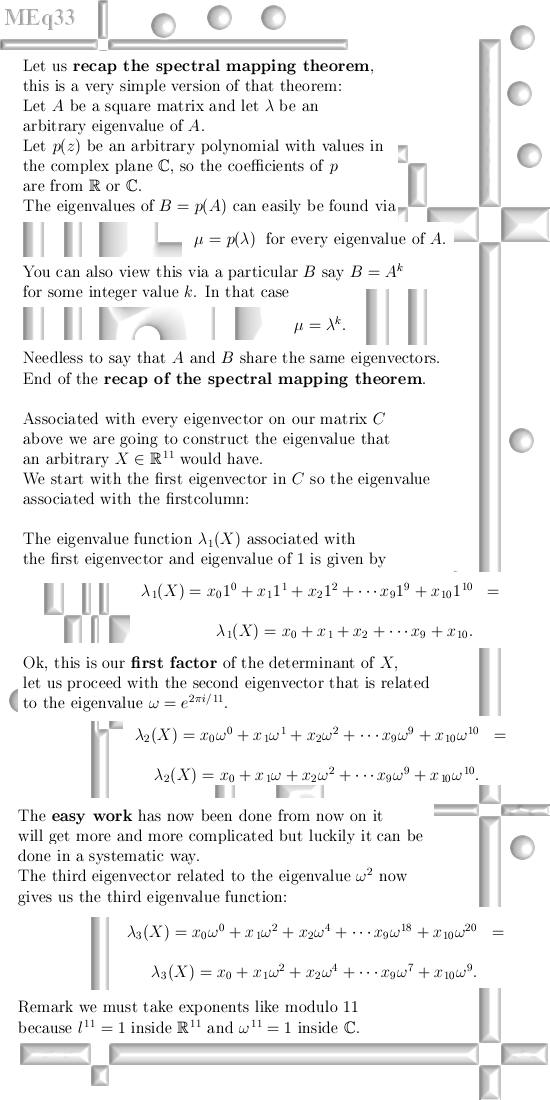
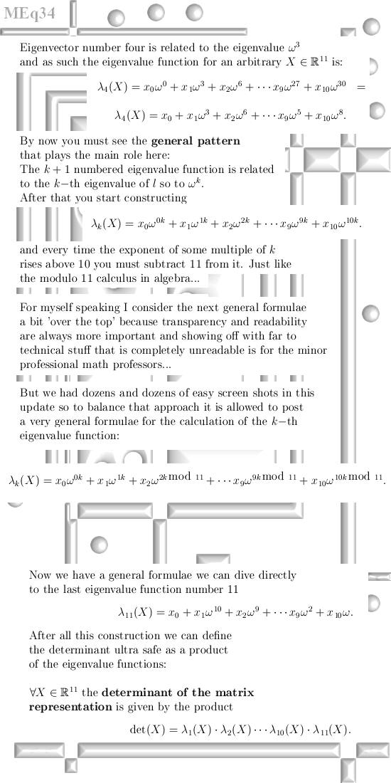
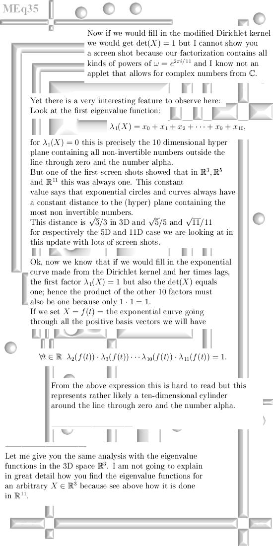
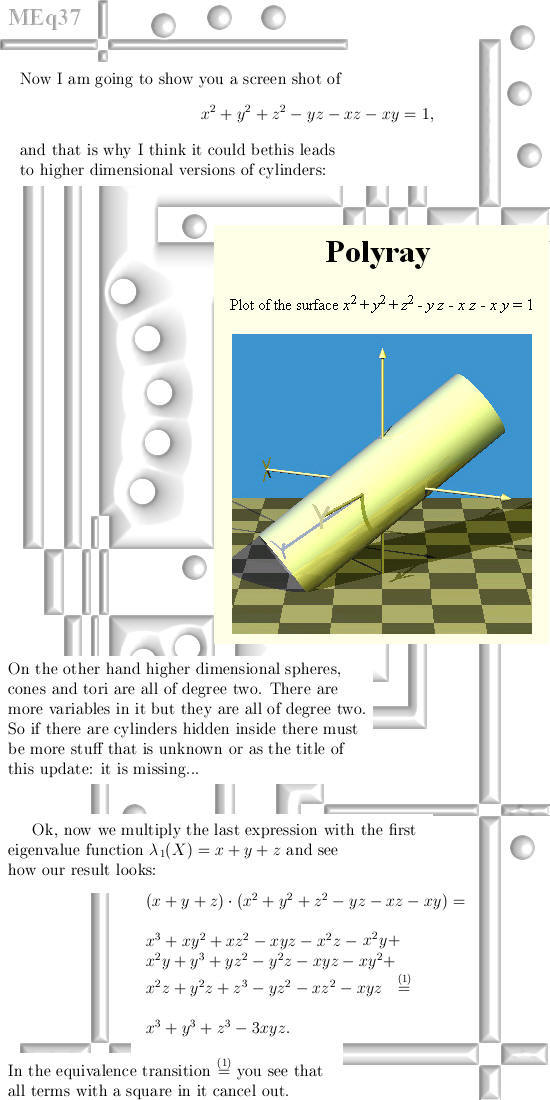
most important results of this year number 2015: The equation that defines that cylinder is a factor of 3D matrix representations of circular numbers. In this appendix I am again using the method of eigenvalue functions, this is a powerful method that by far is not exhausted. In the future we will proceed with that.. Well here is the stuff:
Once more: The fact there is a cylinder hiding inside the equation for the determinant as one of the factors is a crazy result. But I said it so often the last four years: the higher dimensional complex numbers are a giant ocean where the two dimensional complex plane from those 'professional professors' is a small fishbowl.. Till updates.
|
|
From 04
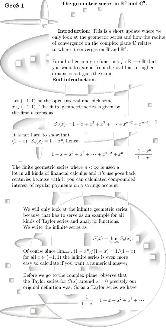
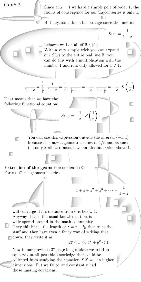
Sept 2015: The geometric series in 3D.
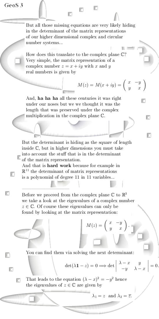
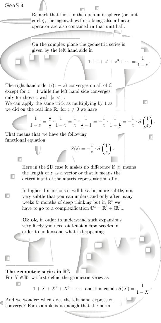
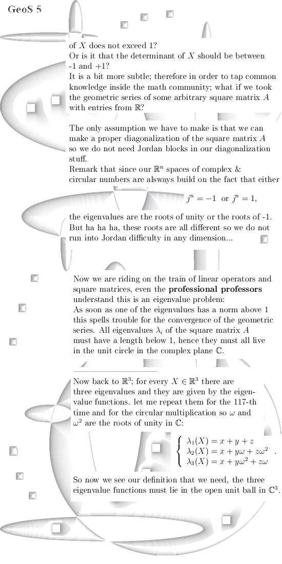
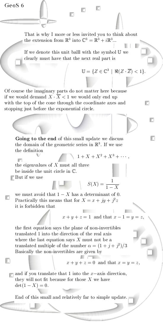
This is a small six page long update and the goal of this update for me was to write a text that could be understood in large part by students of mathematics in their second year. So if you are a student of the science of math, what must you know before you can grasp the butter & meat of this six page small update? Very simple: 1) You must know the complex
plane a bit. So here we go, only six pages (or jpg pictures) long:
Further reading: Geometric
series Ok, end of this update. Live well & work well my dear reader.
|
|
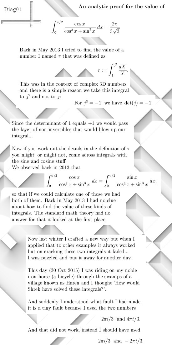
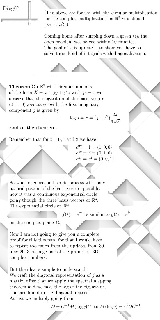
From 21
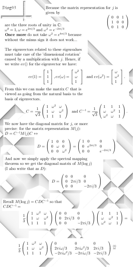
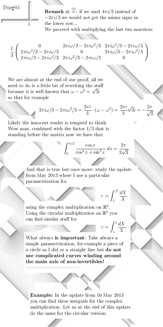
Nov 2015: Integral calculus done with matrix diagonalization.
About two and a half year back I gave the first proof for integrals like below having the analytical value they have, back in the time I named it the principle of massive modified madness. That sounds strange, I understand that, but if you understand the math behind the stuff you also understand humans are only dumb monkeys when it comes to complex numbers... Anyway, to make a long story short, in the next six pages you can find a more elementary proof that does not use ´massive modified madness´ at all but only subtle stuff from inside the toolbox of modern math. All you need is basic insight in what you can do with 3D complex numbers, so good luck with it.
Ok, that was it. It is the year 2015 and there is about zero point zero reaction from the estimated one hundred thousand math professors there are our small planet... Let´s leave it with that, till updates my dear reader.
|
|
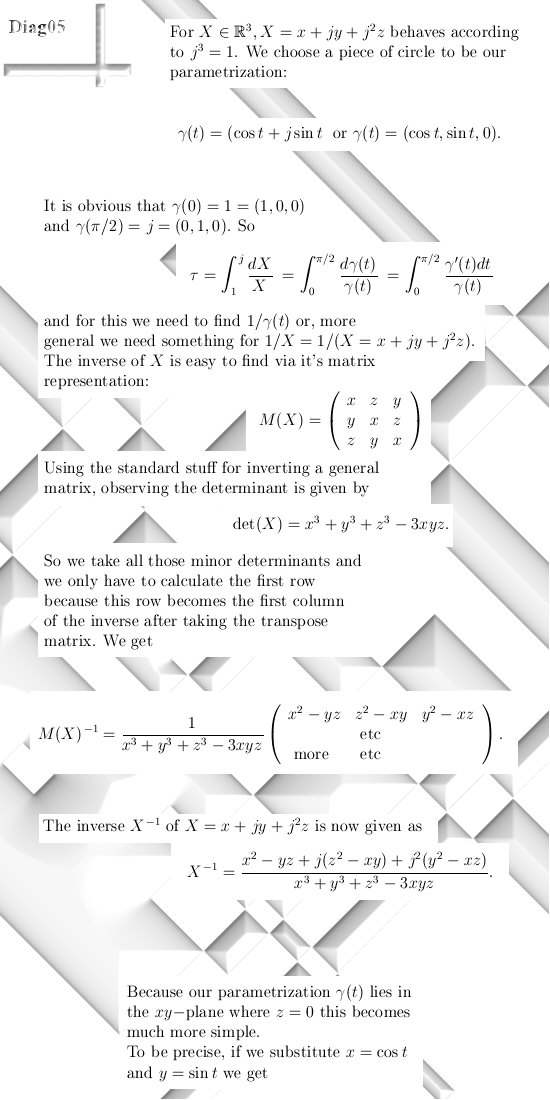
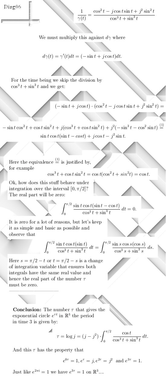
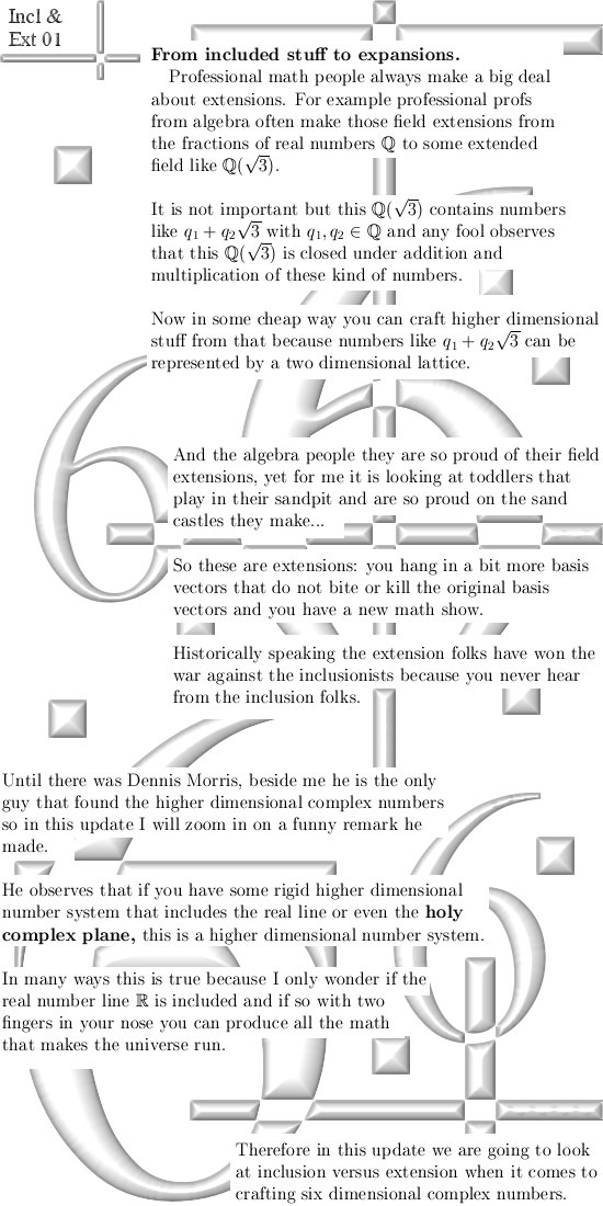
From 06
Dec 2015: This update from 8 pages long is partly based on an idea
from Dennis Morris who wrote a book with the title: Complex numbers the
higher dimensional forms -2nd edition.
For me it is very funny that Dennis
is not a professional math worker, he does physics in particular the quantum
variant as far as I know. Anyway if you are interested you can buy this book
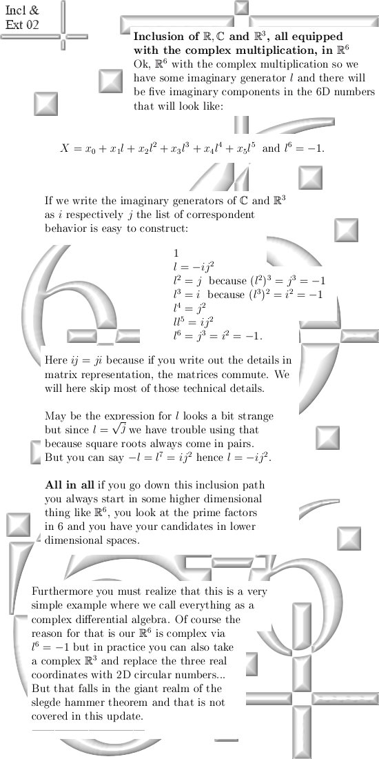
from Amazon. _________ After having said that, in this update I do the following:
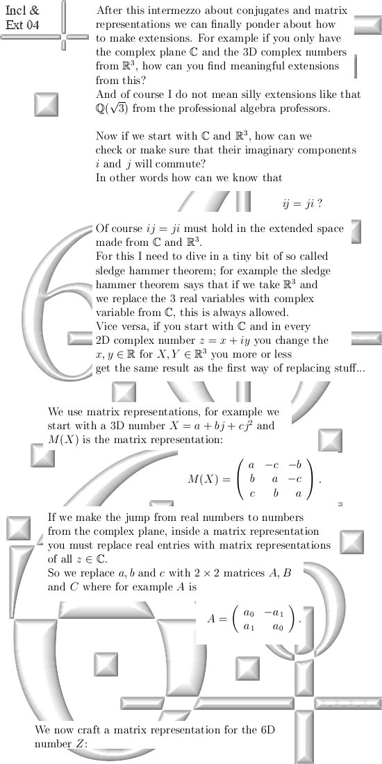
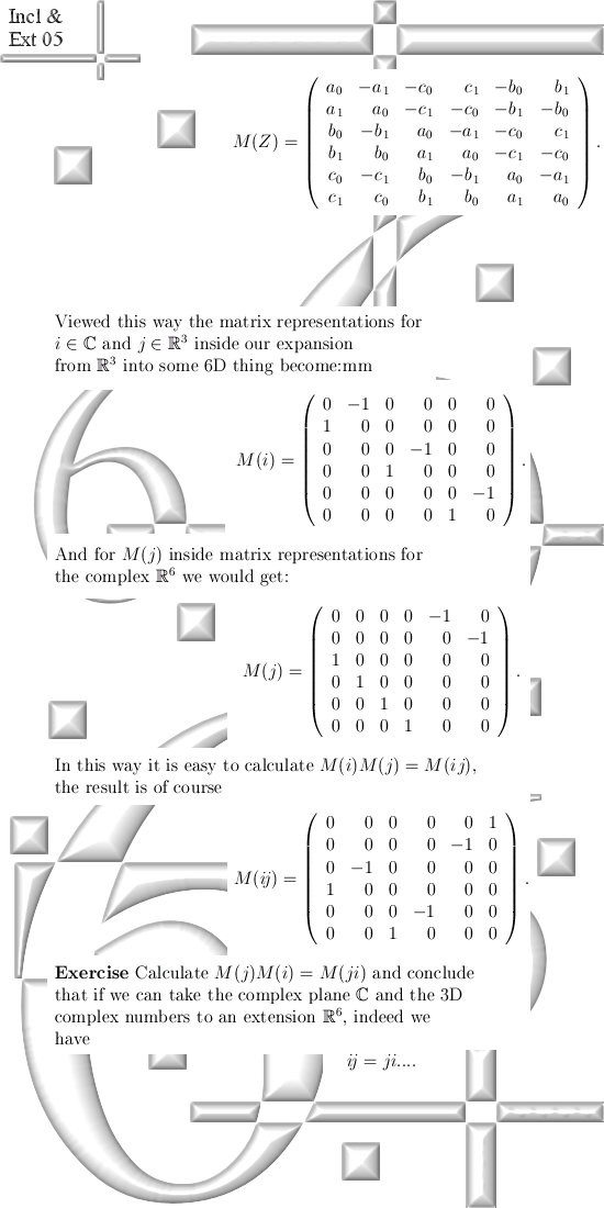
1) We start with 6D complex numbers
and observe that like expected the complex plane is included and the 3D
numbers too. _________ Enough of the bla bla bla, here are 8 fresh pages:
Indeed this is the end of this
update, don´t forget to bookmark my new website 3dcomplexnumbers.net (ok I
am a bit lazy with placing updates over there but it is more or less long
term policy that everything will go over there). Till updates.
|
| From xx xxx 2015: |
|
|
|
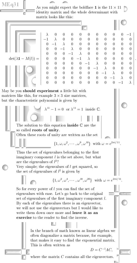
|